Menu
Physics Lesson 3.5.4 - Average and Instantaneous Velocity
Please provide a rating, it takes seconds and helps us to keep this resource free for all to use
Welcome to our Physics lesson on Average and Instantaneous Velocity, this is the fourth lesson of our suite of physics lessons covering the topic of Speed and Velocity in 1 Dimension, you can find links to the other lessons within this tutorial and access additional physics learning resources below this lesson.
Average and Instantaneous Velocity
The approach is the same as for Average and Instantaneous Speed. Thus, Average Velocity < v⃗ > represents the total Displacement divided by the total Time taken. The concept of average velocity is particularly useful when dealing with non-uniform motion.
Mathematically, we have:
As for Instantaneous Velocity v⃗, again we take two neighbouring values for Position and Time. In this way, we obtain one interval for each quantity, namely ∆x⃗ and ∆t. Therefore, we obtain the equation
Example
Calculate the average velocity of the entire motion and the instantaneous velocity at t = 4.0 s for a moving object whose Position vs Time graph is shown in the figure below.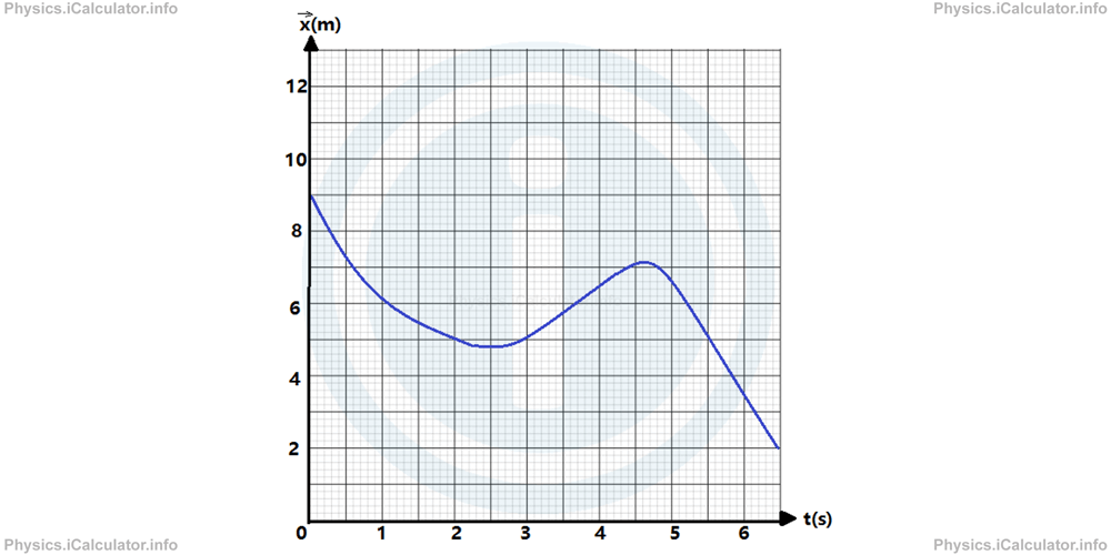
Solution
From the graph, we see that the initial position is x⃗i = 9.0m and the final position is x⃗f = 2.0m, the initial time is ti = 0 and the final time is tf = 6.5s. Therefore, applying the formula of average velocity
we obtain after the substitutions
= 7.0m/6.5s
= 1.1 m/s
(The result is written at one decimal place to fit the clues. Look at the tutorail Significant Figures and Their Importance).
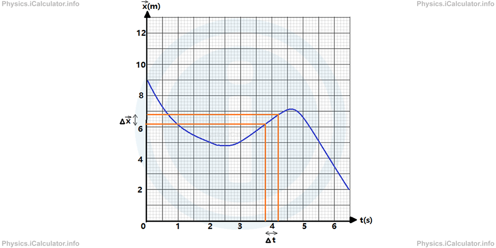
As for the instantaneous velocity at the instant required (at t = 4.0s), again we take two surrounding values for each quantity shown in the graph (two for position and two for the time). These values must be as close as possible to the point required. For example, we can choose t1 = 3.8s and t2 = 4.2s. From the graph, we can see that the corresponding values of position are x⃗1 = 6.2m and x⃗2 = 6.8m as shown below.
Using the equation of the instantaneous velocity
we obtain after substituting the known values:
6.8m - 6.2m/4.2s - 3.8s
= 0.6m/0.4s
= 1.5 m/s
Remark! From Mathematics, it is known that the slope of a graph (otherwise known as gradient) at a certain point is obtained by dividing the change in vertical coordinate to the change in the horizontal one for a small interval surrounding the given point. This can be observed in our example as well. Look at the magnified section of the graph around the instant t = 4.0 s.
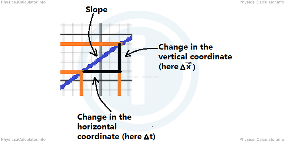
Therefore, we obtain a very important rule in Kinematics:
"The slope (gradient) of the Position vs Time graph gives the Velocity."
This rule helps a lot in understanding the properties of velocity and gives it a mathematical meaning.
You have reach the end of Physics lesson 3.5.4 Average and Instantaneous Velocity. There are 4 lessons in this physics tutorial covering Speed and Velocity in 1 Dimension, you can access all the lessons from this tutorial below.
More Speed and Velocity in 1 Dimension Lessons and Learning Resources
Whats next?
Enjoy the "Average and Instantaneous Velocity" physics lesson? People who liked the "Speed and Velocity in 1 Dimension lesson found the following resources useful:
- Average Instantaneous Velocity Feedback. Helps other - Leave a rating for this average instantaneous velocity (see below)
- Kinematics Physics tutorial: Speed and Velocity in 1 Dimension. Read the Speed and Velocity in 1 Dimension physics tutorial and build your physics knowledge of Kinematics
- Kinematics Revision Notes: Speed and Velocity in 1 Dimension. Print the notes so you can revise the key points covered in the physics tutorial for Speed and Velocity in 1 Dimension
- Kinematics Practice Questions: Speed and Velocity in 1 Dimension. Test and improve your knowledge of Speed and Velocity in 1 Dimension with example questins and answers
- Check your calculations for Kinematics questions with our excellent Kinematics calculators which contain full equations and calculations clearly displayed line by line. See the Kinematics Calculators by iCalculator™ below.
- Continuing learning kinematics - read our next physics tutorial: Speed and Velocity in 2 and 3 Dimensions
Help others Learning Physics just like you
Please provide a rating, it takes seconds and helps us to keep this resource free for all to use
We hope you found this Physics lesson "Speed and Velocity in 1 Dimension" useful. If you did it would be great if you could spare the time to rate this physics lesson (simply click on the number of stars that match your assessment of this physics learning aide) and/or share on social media, this helps us identify popular tutorials and calculators and expand our free learning resources to support our users around the world have free access to expand their knowledge of physics and other disciplines.